6. LaTeX usage

Asymptote comes with a convenient LaTeX style file asymptote.sty that makes LaTeX Asymptote-aware. Entering Asymptote code directly into the LaTeX source file, at the point where it is needed, keeps figures organized and avoids the need to invent new file names for each figure. Simply add the line \usepackage{asymptote} at the beginning of your file and enclose your Asymptote code within a \begin{asy}...\end{asy} environment. As with the LaTeX comment environment, the \end{asy} command must appear on a line by itself, with no leading spaces or trailing commands/comments.

The current version of asymptote.sty even supports the direct embedding of 3D PRC files within LaTeX. The sample LaTeX file below, named latexusage.tex, can be run as follows:

latex latexusage
asy latexusage
latex latexusage

or

pdflatex latexusage
asy latexusage
pdflatex latexusage

To switch between using latex and pdflatex you may first need to remove the files latexusage_.* and latexusage.aux.

If the inline option is given to the asymptote.sty package, inline LaTeX code is generated instead of EPS or PDF files. This makes LaTeX symbols visible to the \begin{asy}...\end{asy} environment. In this mode, Asymptote correctly aligns LaTeX symbols defined outside of \begin{asy}...\end{asy}, but treats their size as zero; an optional second string can be given to Label to provide an estimate of the unknown label size.

Note that if latex is used with the inline option, the labels might not show up in DVI viewers that cannot handle raw PostScript code. One can use dvips/dvipdf to produce PostScript/PDF output (we recommend using the modified version of dvipdf in the Asymptote patches directory, which accepts the dvips -z hyperdvi option).

An excellent tutorial by Dario Teixeira on integrating Asymptote and LaTeX is available at http://dario.dse.nl/projects/asylatex/.

Here now is latexusage.tex:

\documentclass[12pt]{article}

% Use this form to include eps (latex) or pdf (pdflatex) files:
\usepackage{asymptote}

% Use this form with latex or pdflatex to include inline LaTeX code:
%\usepackage[inline]{asymptote}

% Enable this line to produce pdf hyperlinks with latex:
%\usepackage[hypertex]{hyperref}

% Enable this line to produce pdf hyperlinks with pdflatex:
%\usepackage[pdftex]{hyperref}

\begin{document}

\begin{asydef}
// Global Asymptote definitions can be put here.
usepackage("bm");
texpreamble("\def\v#1{\bm{#1}}");
\end{asydef}

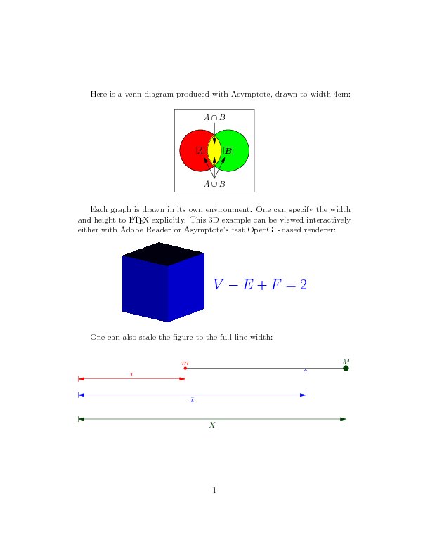
Here is a venn diagram produced with Asymptote, drawn to width 4cm:

\def\A{A}
\def\B{\v{B}}

%\begin{figure}
\begin{center}
\begin{asy}
size(4cm,0);
pen colour1=red;
pen colour2=green;

pair z0=(0,0);
pair z1=(-1,0);
pair z2=(1,0);
real r=1.5;
path c1=circle(z1,r);
path c2=circle(z2,r);
fill(c1,colour1);
fill(c2,colour2);

picture intersection=new picture;
fill(intersection,c1,colour1+colour2);
clip(intersection,c2);

add(intersection);

draw(c1);
draw(c2);

//draw("$\A$",box,z1);              // Requires [inline] package option.
//draw(Label("$\B$","$B$"),box,z2); // Requires [inline] package option.
draw("$A$",box,z1);            
draw("$\v{B}$",box,z2);

pair z=(0,-2);
real m=3;
margin BigMargin=Margin(0,m*dot(unit(z1-z),unit(z0-z)));

draw(Label("$A\cap B$",0),conj(z)--z0,Arrow,BigMargin);
draw(Label("$A\cup B$",0),z--z0,Arrow,BigMargin);
draw(z--z1,Arrow,Margin(0,m));
draw(z--z2,Arrow,Margin(0,m));

shipout(bbox(0.25cm));
\end{asy}
%\caption{Venn diagram}\label{venn}
\end{center}
%\end{figure}

Each graph is drawn in its own environment. One can specify the width
and height to \LaTeX\ explicitly. This 3D example can be viewed
interactively either with Adobe Reader or Asymptote's fast OpenGL-based
renderer:
\begin{center}
\begin{asy}[0,4cm]
import three;
if(settings.render < 0) settings.render=8;

draw(unitcube,blue);
label("$V-E+F=2$",(0,1,0.5),3Y,blue+fontsize(20));
\end{asy}
\end{center}

One can also scale the figure to the full line width:
\begin{center}
\begin{asy}[\the\linewidth]
pair z0=(0,0);
pair z1=(2,0);
pair z2=(5,0);
pair zf=z1+0.75*(z2-z1);

draw(z1--z2);
dot(z1,red+0.15cm);
dot(z2,darkgreen+0.3cm);
label("$m$",z1,1.2N,red);
label("$M$",z2,1.5N,darkgreen);
label("$\hat{\ }$",zf,0.2*S,fontsize(24)+blue);

pair s=-0.2*I;
draw("$x$",z0+s--z1+s,N,red,Arrows,Bars,PenMargins);
s=-0.5*I;
draw("$\bar{x}$",z0+s--zf+s,blue,Arrows,Bars,PenMargins);
s=-0.95*I;
draw("$X$",z0+s--z2+s,darkgreen,Arrows,Bars,PenMargins);
\end{asy}
\end{center}
\end{document}